| Grid characteristics | ||||||||||
|---|---|---|---|---|---|---|---|---|---|---|
| Grid | Level |
Cells
|
Cell Spacing
|
Max distortion
|
||||||
| #Cells | Cell Area | Defect | Min | Mean | Max | Area | Radial | Edge | ||
| IVEA | 5 | 2432 | 209,907 km² | 1.20 | −41.63 | 494.00 | +47.73 | 1.36% | 28.78% | 13.42% |
| IVEA | 6 | 7292 | 69,968 km² | 1.20 | −28.16 | 285.28 | +23.32 | 1.37% | 31.62% | 12.77% |
| IVEA | 7 | 21872 | 23,323 km² | 1.20 | −13.99 | 164.74 | +16.56 | 1.36% | 28.79% | 13.04% |
| IVEA | 8 | 65612 | 7,774 km² | 1.20 | −9.41 | 95.11 | +8.06 | 1.37% | 31.42% | 12.51% |
| IVEA | 9 | 196832 | 2,591 km² | 1.20 | −4.67 | 54.92 | +5.60 | 1.36% | 28.70% | 12.81% |
| ISEA (DGGAL) | 5 | 2432 | 209,909 km² | 1.21 | −42.94 | 494.94 | +66.80 | 1.47% | 29.91% | 15.15% |
| ISEA (DGGAL) | 6 | 7292 | 69,968 km² | 1.20 | −37.79 | 285.64 | +26.40 | 1.36% | 36.21% | 14.95% |
| ISEA (DGGAL) | 7 | 21872 | 23,323 km² | 1.21 | −14.41 | 165.06 | +23.30 | 1.48% | 29.68% | 15.31% |
| ISEA (DGGAL) | 8 | 65612 | 7,774 km² | 1.20 | −13.28 | 95.26 | +9.66 | 1.36% | 35.79% | 14.34% |
| ISEA (DGGAL) | 9 | 196832 | 2,591 km² | 1.21 | −4.81 | 55.02 | +8.24 | 1.48% | 29.48% | 15.14% |
| ISEA (dggridR) | 5 | 2432 | 210,035 km² | 1.41 | −58.11 | 494.01 | +50.42 | 2.07% | 12.74% | 15.10% |
| ISEA (dggridR) | 6 | 7292 | 69,965 km² | 1.16 | −34.66 | 285.51 | +22.09 | 4.11% | 14.72% | 14.92% |
| ISEA (dggridR) | 7 | 21872 | 23,324 km² | 1.42 | −19.55 | 164.91 | +20.63 | 2.03% | 14.17% | 15.29% |
| ISEA (dggridR) | 8 | 65612 | 7,774 km² | 1.16 | −12.31 | 95.24 | +8.60 | 4.11% | 14.28% | 14.33% |
| ISEA (dggridR) | 9 | 196832 | 2,591 km² | 1.43 | −6.54 | 55.00 | +7.50 | 2.02% | 14.69% | 15.13% |
| FULLER (dggridR) | 5 | 2432 | 209,966 km² | 1.29 | −67.30 | 493.38 | +28.23 | 11.47% | 10.85% | 11.80% |
| FULLER (dggridR) | 6 | 7292 | 69,986 km² | 1.47 | −41.21 | 284.99 | +21.90 | 12.26% | 10.78% | 11.05% |
| FULLER (dggridR) | 7 | 21872 | 23,323 km² | 1.29 | −23.32 | 164.58 | +9.04 | 12.75% | 10.73% | 11.10% |
| FULLER (dggridR) | 8 | 65612 | 7,774 km² | 1.48 | −14.00 | 95.03 | +7.33 | 13.01% | 10.89% | 10.98% |
| FULLER (dggridR) | 9 | 196832 | 2,591 km² | 1.29 | −7.86 | 54.87 | +3.01 | 13.18% | 10.65% | 10.78% |
| fuller-uniform | 5 | 2252 | 226,633 km² | 1.13 | −42.77 | 513.02 | +39.46 | 11.64% | 1.56% | 39.38% |
| fuller-uniform | 6 | 6762 | 75,447 km² | 1.13 | −24.77 | 296.06 | +22.80 | 12.34% | 0.95% | 39.62% |
| fuller-uniform | 7 | 23042 | 22,138 km² | 1.13 | −13.43 | 160.38 | +12.36 | 12.85% | 0.53% | 39.67% |
| fuller-uniform | 8 | 72252 | 7,060 km² | 1.13 | −7.59 | 90.57 | +6.98 | 13.08% | 0.31% | 39.69% |
| fuller-uniform | 9 | 163842 | 3,113 km² | 1.13 | −5.04 | 60.15 | +4.64 | 13.19% | 0.20% | 39.73% |
Global Grids for Spatial Analysis
Overview
Uniform spatial data binning is a core challenge for global geospatial studies (for example, in environmental or social sciences). The purpose of data binning is to split the data into roughly comparable regions (grid cells), allowing one to apply traditional statistical techniques, such as regression analysis, to the resulting structured dataset. Popular binning methods such as equal-degree grids (where the Earth’s surface is split into square cells of fixed angular size) do not result in uniform distributions since the actual shape and dimension of the cell depends on its geographic location. For instance, cells in the Northern Hemisphere can be two to three times larger (by surface area) compared to cells located near the equator despite having identical angular measurements. Various global discrete grid systems have been proposed in the literature and the industry to facilitate spatial data binning. These systems rely on complex mathematical transformations in order to create grids with nearly uniform distribution on the spheroid.
Goodchild Criteria1,2 describe the common desiderata for high-quality global grid systems. These include regularity (consistent spatial arrangement of cells), equal-area partitioning (cells should cover approximately the same surface area), and equal spacing of cell centroids to minimize distortions in distance-based computations. The cells of a hypothetical ideal grid system would perfectly approximate equally-spaced homogenous geodesic circles on the Earth’s surface. Since topological constraints make it impossible to create a grid that can satisfy all the conditions simultaneously, practical grid construction is a balancing exercise.
Hexagonal grids are of particular interest. Hexagons are one of the few shapes that allow perfect tiling. Of all these shapes, hexagons maximize the surface area covered by each cell. Each hexagon has exactly six direct neighbors, which is the maximal number for any regular polygon. Furthermore, centroids of neighboring cells are equidistant, and their shared edges have the same length. This makes hexagonal grids ideal for modeling spatial processes (regular connectivity translates to equal transition probabilities under a neutral model). At the same time, the topological properties of the sphere make it impossible to construct a uniform spherical hexagonal grid.
To absorb the excess curvature, additional shapes must be introduced. The minimal amount is 12 pentagons, which is the approach used in modern icosahedral grids discussed here. Pentagonal cells introduce “defects” in the grid. In practice, these defects are negligible since they are limited to only 12 cells out of thousands and are usually located sufficiently far away from typical areas of interest. One can further minimize the defect by aiming to maximize the pentagon-to-hexagon area ratio. For optimal grids, this ratio is 5/6 (improving it further is not possible without introducing additional distortion).
The goal of this experiment is to survey the characteristics of available grid systems and present arguments for their adoption in global geospatial studies. We only consider hexagonal grids. In particular, we focus on the novel IVEA (Icosahedral Vertex-Oriented Great Circle Equal Area) grid implemented in the DGGAL library3.
Grid Systems
The following grids and grid implementations are considered:
Discrete Global Grid Abstraction Library3 — a new open-source library that implements and further improves several well-known grid systems. The principal author of
DGGAL(Jérôme St-Louis) is an advocate of Open Standards in Discrete Global Grid Systems and a contributor to OGC standards. Of particular interest to our experiment are theIVEA3HandISEA3Hgrid systems. Both these models rely on the recursive subdivision of a regular icosahedron to produce hexagonal regions and project them to the sphere.ISEA3His based on a well-known Snyder Equal-Area Projection4 and is a known gold standard among uniform global grids.IVEA3His a modification of the Snyder construction, utilizing a different face partitioning method5 that further enhances grid uniformity.Discrete Global Grid Generation Software6 via the R package
dggridR7. We are evaluating the hexagonal aperture-3ISEA(Snyder projection) andFuller(Gray-Fuller projection8) grids. The specification of the ISEA grid should be equivalent to the one used byDGGAL, and it will be interesting to compare the two implementations.Uniform Fuller-Gray Grid9 — a spatial grid that utilizes the Fuller-Gray projection8, initially implemented by10. Rather than relying on the recursive subdivision of the surface, this method generates equidistant points on a planar triangle and projects them onto the sphere to construct uniformly distributed cell centroids. The cell shapes are then constructed as the Voronoi tesselation of the sphere. The advantage of this method is that it allows flexible grid resolution selection, unlike the common DGGRS systems, which are limited to a constrained resolution hierarchy.
All the surveyed grids can be constructed at various resolutions. DGGAL and dggridR support a constrained resolution hierarchy, with cells at each level being approximately 3 times smaller compared to the cells at the previous level. Not all grid resolutions are of practical use for global geospatial studies. We limit our experiments to a set of resolutions between 900km and 60km that are supported by all the grid systems in the survey.
Methods
Grid Construction
Each of the grids is built using the respective tool or library and transformed into a format that allows comparison. We represent each grid as a table, with one row per grid cell. The R code used to construct each grid can be found in R/.
For each cell, we report
- the unique cell identifier in the grid
- the cell centroid
- the cell shape (pentagon or hexagon)
- the cell neighbors and the geodesic segment representing the shared boundary
- the cell geometry (as a geodesic polygon)
DGGAL produces refined edges to more accurately represent the curvature of the projected regions. This means that DGGAL cell geometry is complex polygons that approximate the target hexagonal and pentagonal shapes as constructed by the equal area projection. A higher degree of refinement produces more uniform results at the cost of additional memory and processing. We found the refinement level of 5 to be a reasonable tradeoff between accuracy and computation. This yields around 30 vertices per polygon.
As dggridR does not report cell adjacency, we use a simple brute-force search to identify the nearest cells. While not computationally efficient, this approach is practical enough for one-time grid construction at the target resolutions.
Grid Distortion Analysis
To evaluate the grid uniformity, I consider the following properties:
The maximal area distortion, calculated as the relative difference between the largest cell and the smallest cell (pentagons excluded). This represents the full range of area variability in the grid. For area-uniform grids, this should be close to zero.
The average maximal radial distortion, calculated as the relative difference between the largest and the smallest cell radii (distance from the cell center to its vertices) and averaged across the cells. High radial distortion indicates that a cell is squished or skewed. The radial distortion of a regular polygon is zero.
The average maximal edge distortion, calculated as the relative difference between the longest and the shortest cell edge (distance between two adjacent vertices) and averaged across the cells. High edge distortion indicates unequal connectivity between adjacent cells. The edge distortion of a regular hexagonal grid is zero.
The distance between the centroids of adjacent cells, averaged across cells (min, max, mean). On a uniform grid, the difference between min and max should be zero.
The area defect of the pentagonal cells relative to the average hexagonal cell. In an optimal hexagonal grid on a sphere, this should be \(6/5\) (or lower, at the cost of higher distortion elsewhere)
These metrics aim to capture maximal distortion in key areas across the grid. The motivation for looking at extremes rather than averages is that we are interested in finding a grid that has good properties everywhere as opposed to mostly good properties.
The most important criteria for choosing a grid system are area uniformity and cell spacing uniformity (to ensure that the data is binned equally). Low edge length distortion indicates symmetrical connectivity between the cells (an equal portion of the border shared with each of the neighbors), which is desirable for modeling spatial processes (symmetrical connectivity translates to equal transition probabilities in a neutral model). Finally, low radial distortion indicates regular cell shapes and ensures equal sampling around the cell center.
Results
Grid evaluation results are presented in Table 1
IVEA grids consistently outperform other grids in all criteria except radial distortion. This distortion is the result of the cell squishing that the grid utilizes to equally distribute the excess curvature. It is the only grid family in our survey that consistently maintains an area distortion of less than \(1.5\%\) across the hexagonal cells (and under \(1\%\) area distortion for \(90\%\) of cells) while achieving the optimal pentagon-to-hexagon ratio of \(5/6\). IVEA grids also show the lowest variability in between-cell spacing (along with the Gray-Fuller uniform grid).
ISEA grids are a de-facto gold standard of uniform global grids and perform very well in our tests. The grids generated by dggridR software show slightly less shape and spacing distortion compared to the grids generated by DGGAL, at the expense of area uniformity. Visual inspection (see below) additionally shows differences in how the distortions are distributed across the grid. In dggridR grids, the distortion appears to be more localized, resulting in local discontinuities, while DGGAL generally smoothes out the distortion across a region.
The Gray-Fuller uniform grid exhibits high radial symmetry and low variability in between-cell spacing, which comes at the expense of the higher area distortion. Additionally, the edge length variability is the highest among all surveyed grids, indicating asymmetrically distorted cells.
Grid Characteristics Visualized
The characteristics of some of the grids are visualized below. I focus on relative area, shape, and spacing variability across the grid cells. For practical purposes, I use a grid resolution of ~ 600 km (level 6 for aperture-3 icosahedral grids).
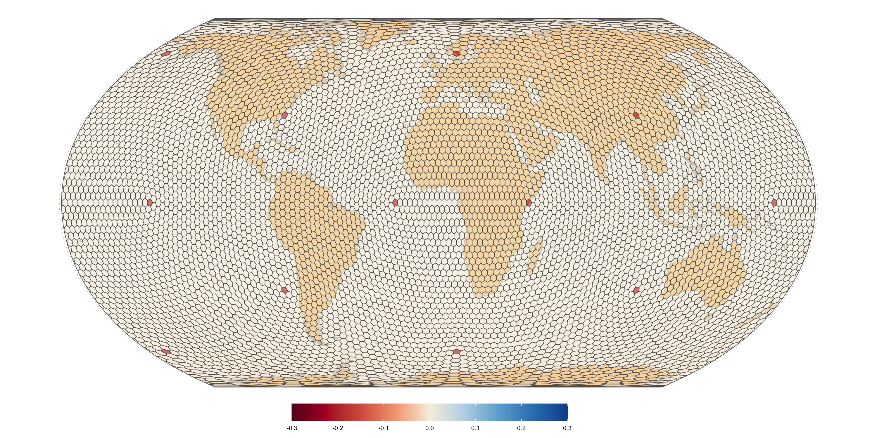
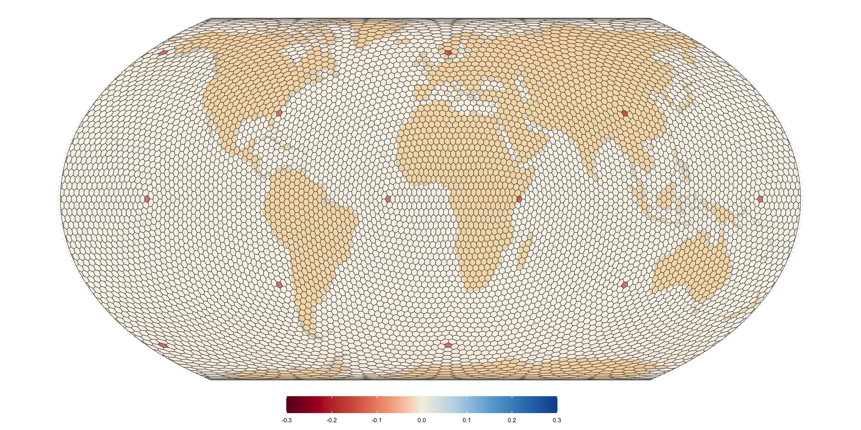
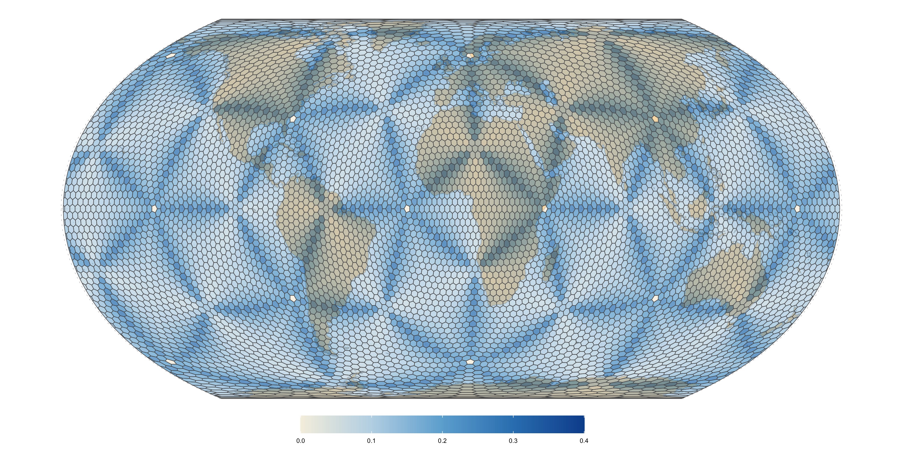
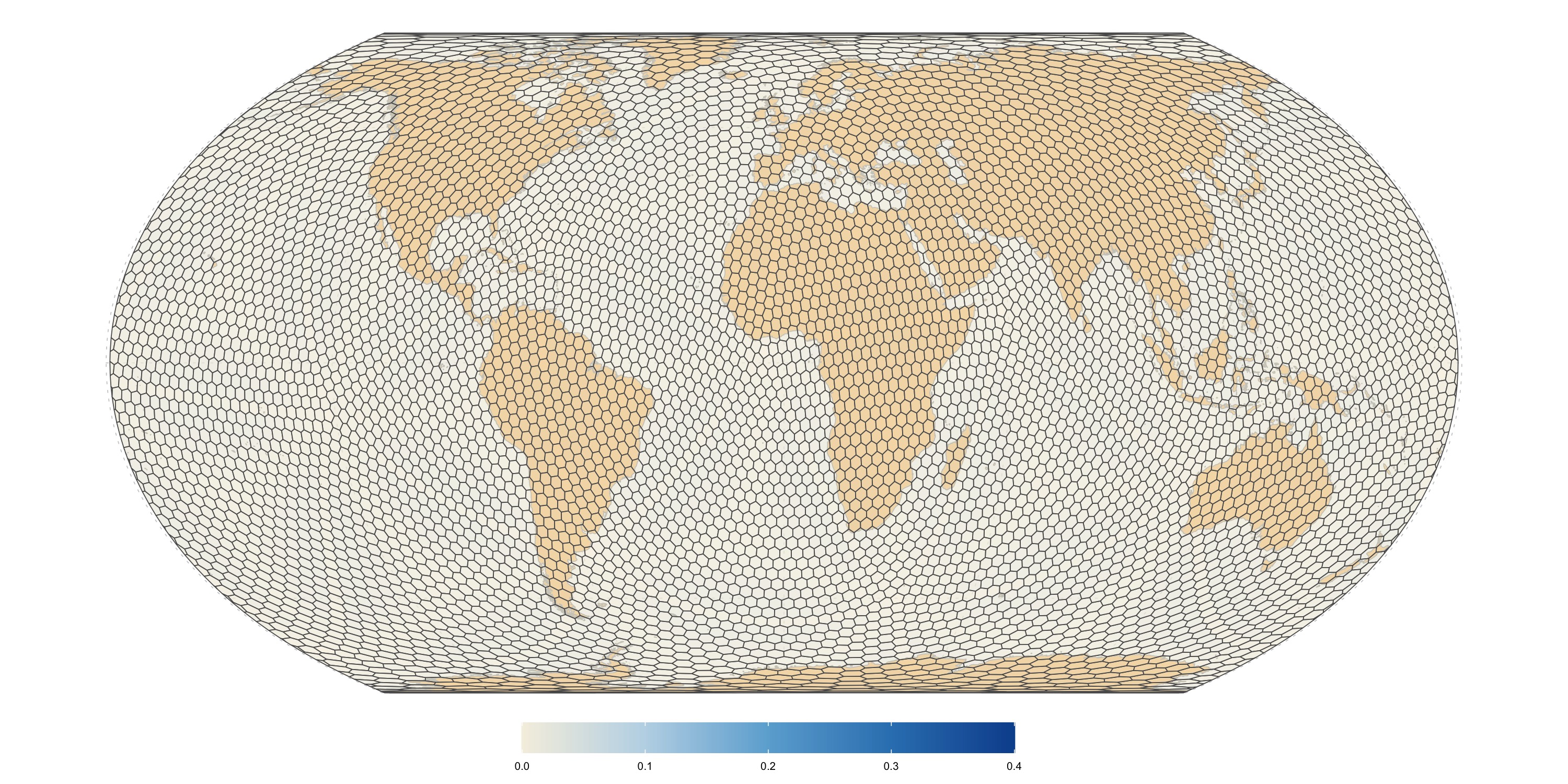
IVEA (DGGAL) level 6 grid
Area distortion relative to the mean. Values closer to zero mean less relative distortion.
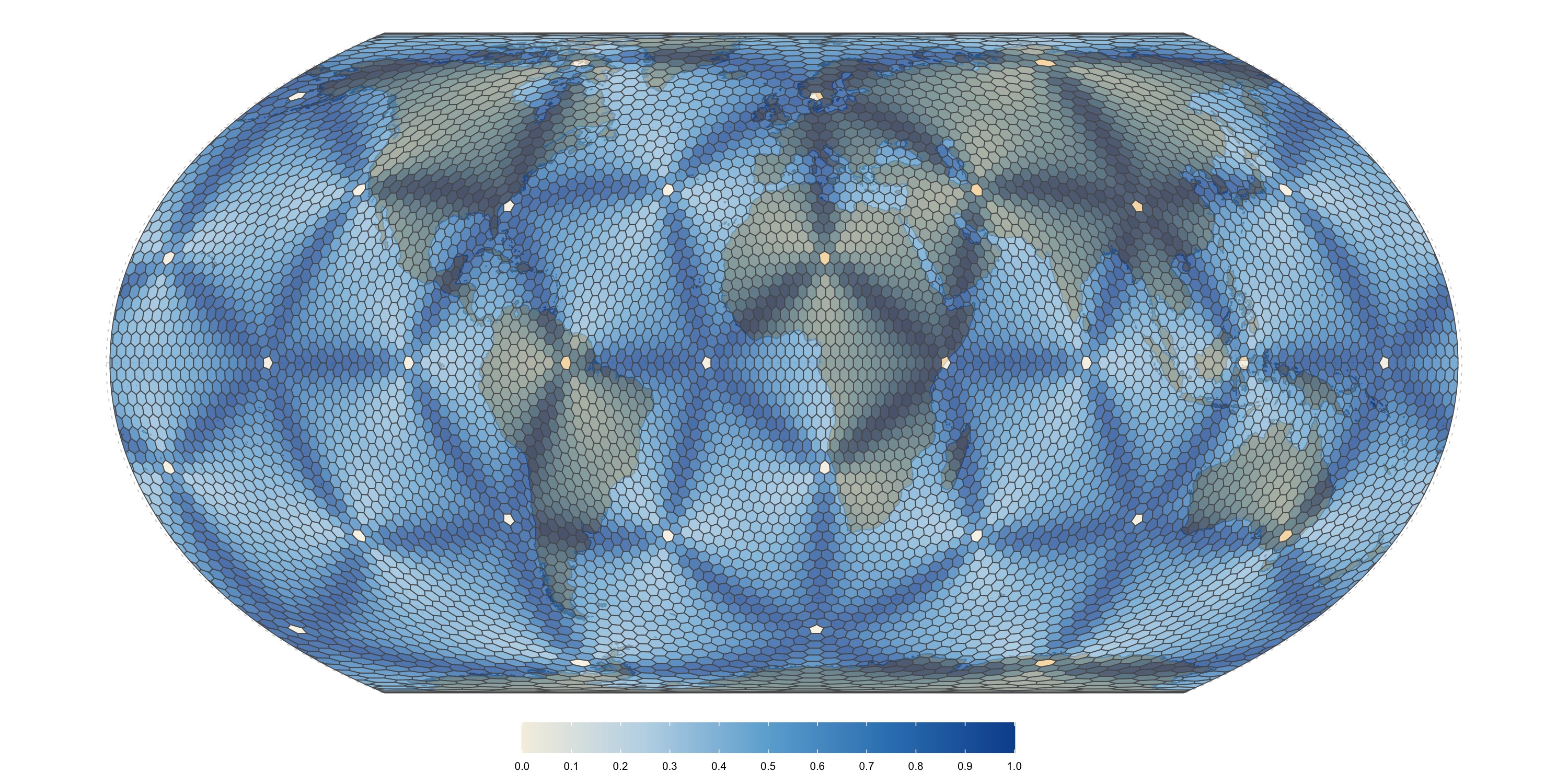
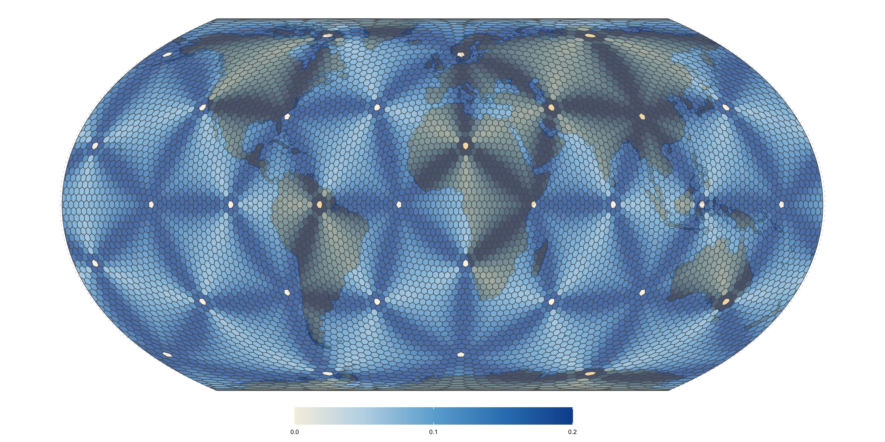
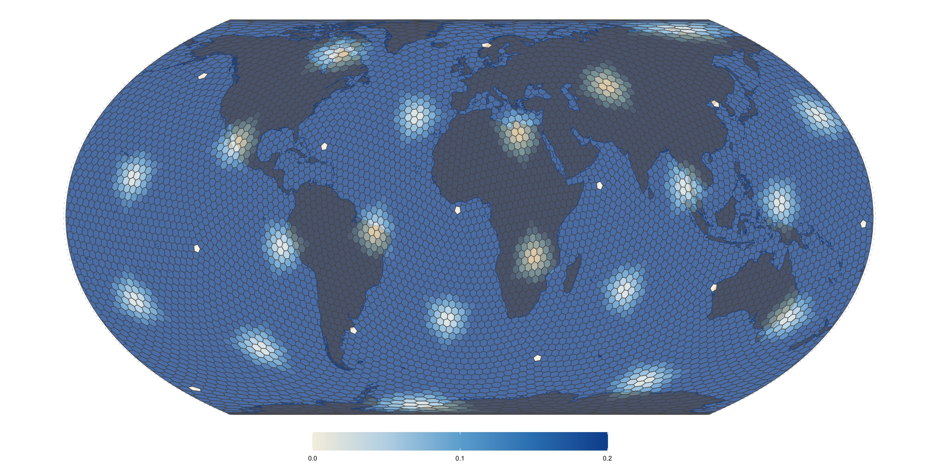
Radial distortion calculated as ratio of largest to smallest distances between the centroid and the base cell boundary vertices, minus one. Zero means perfect radial symmetry.
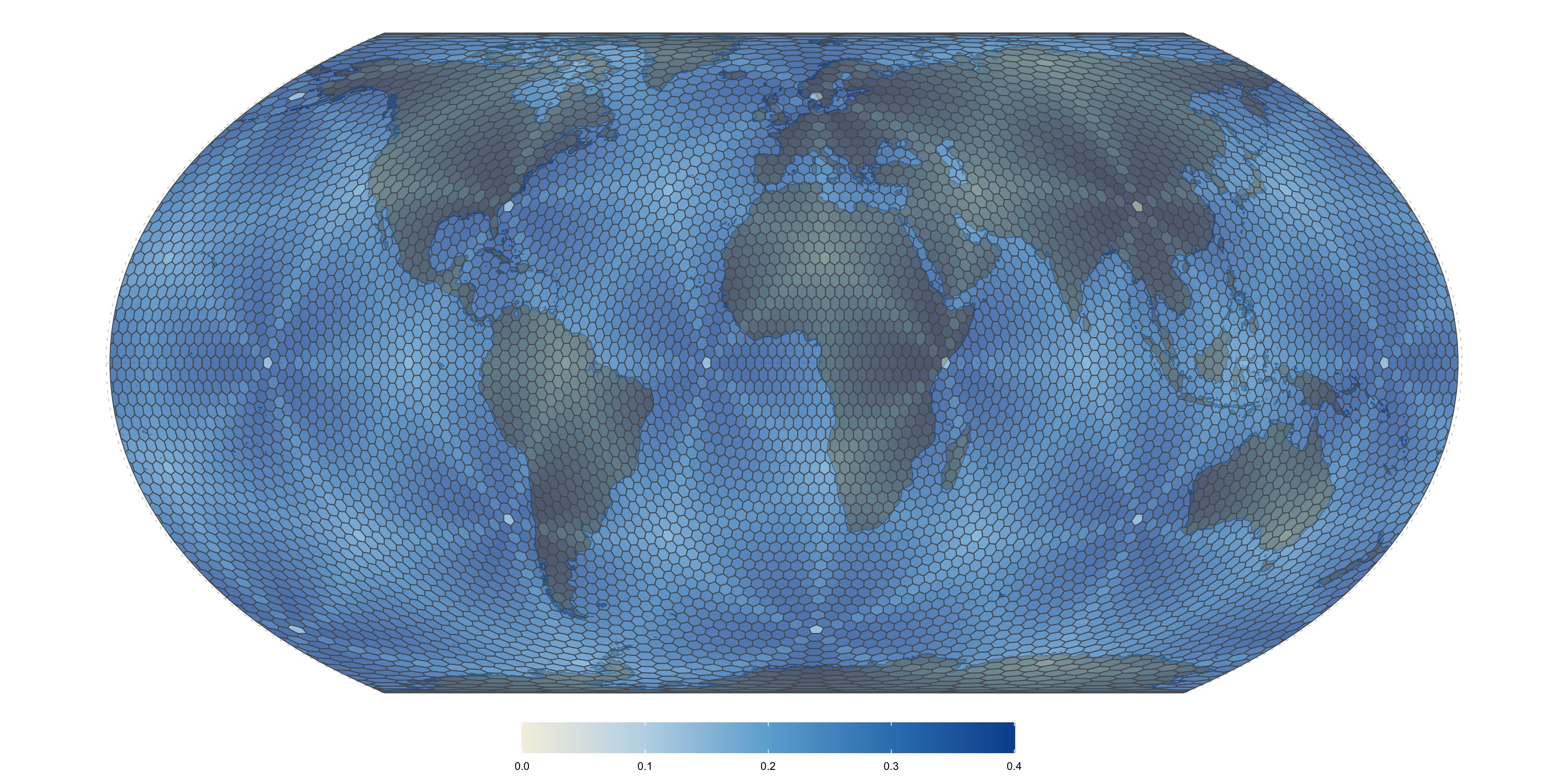
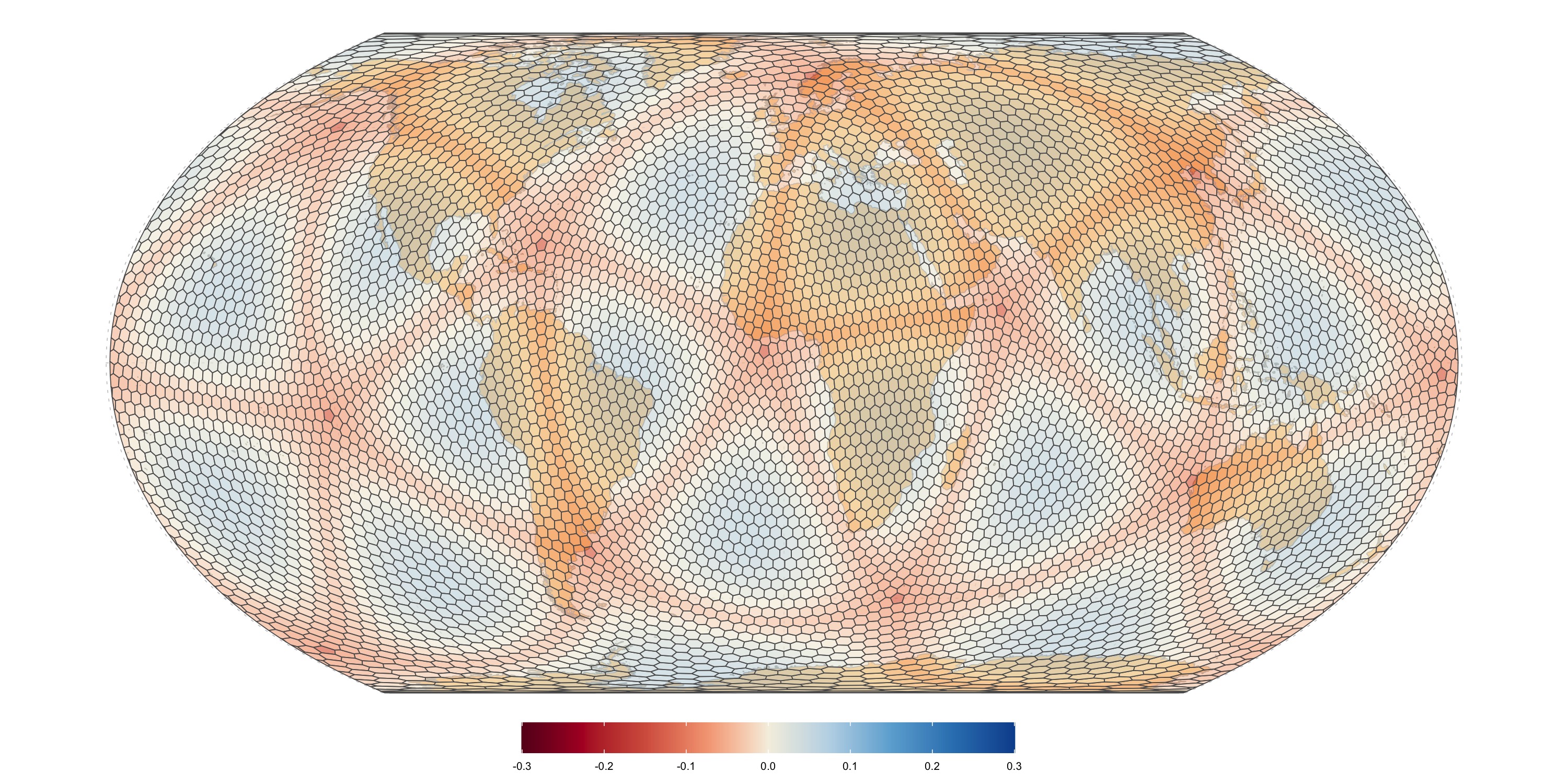
Edge length distortion calculated as ratio of largest to smallest distances between adjacent base cell boundary vertices, minus one. Zero means that all edges have the same length.
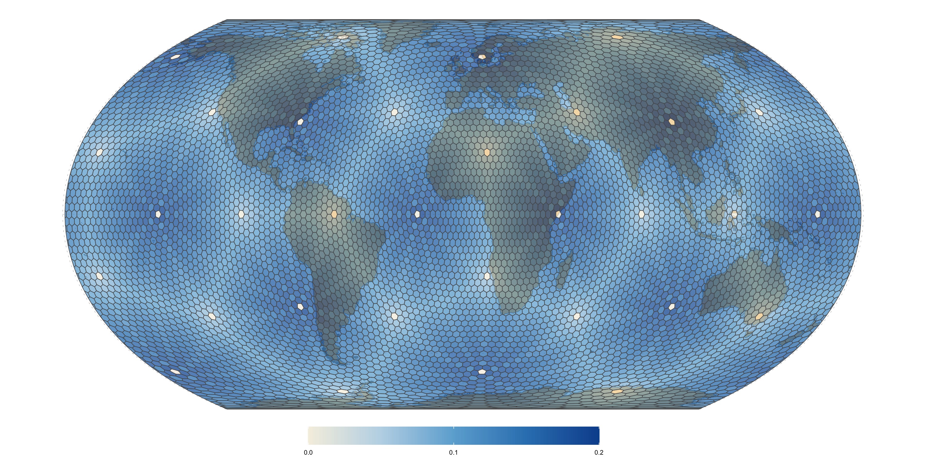
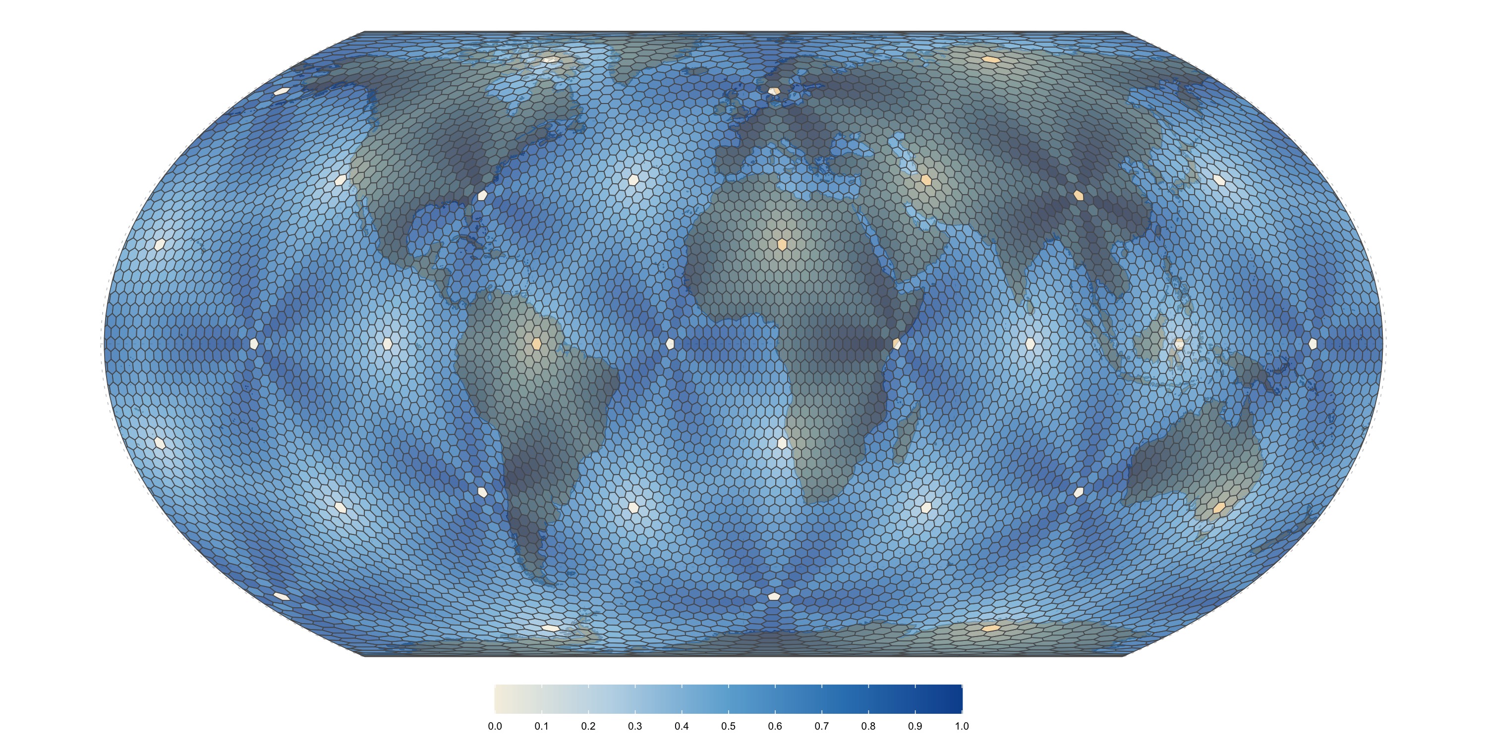
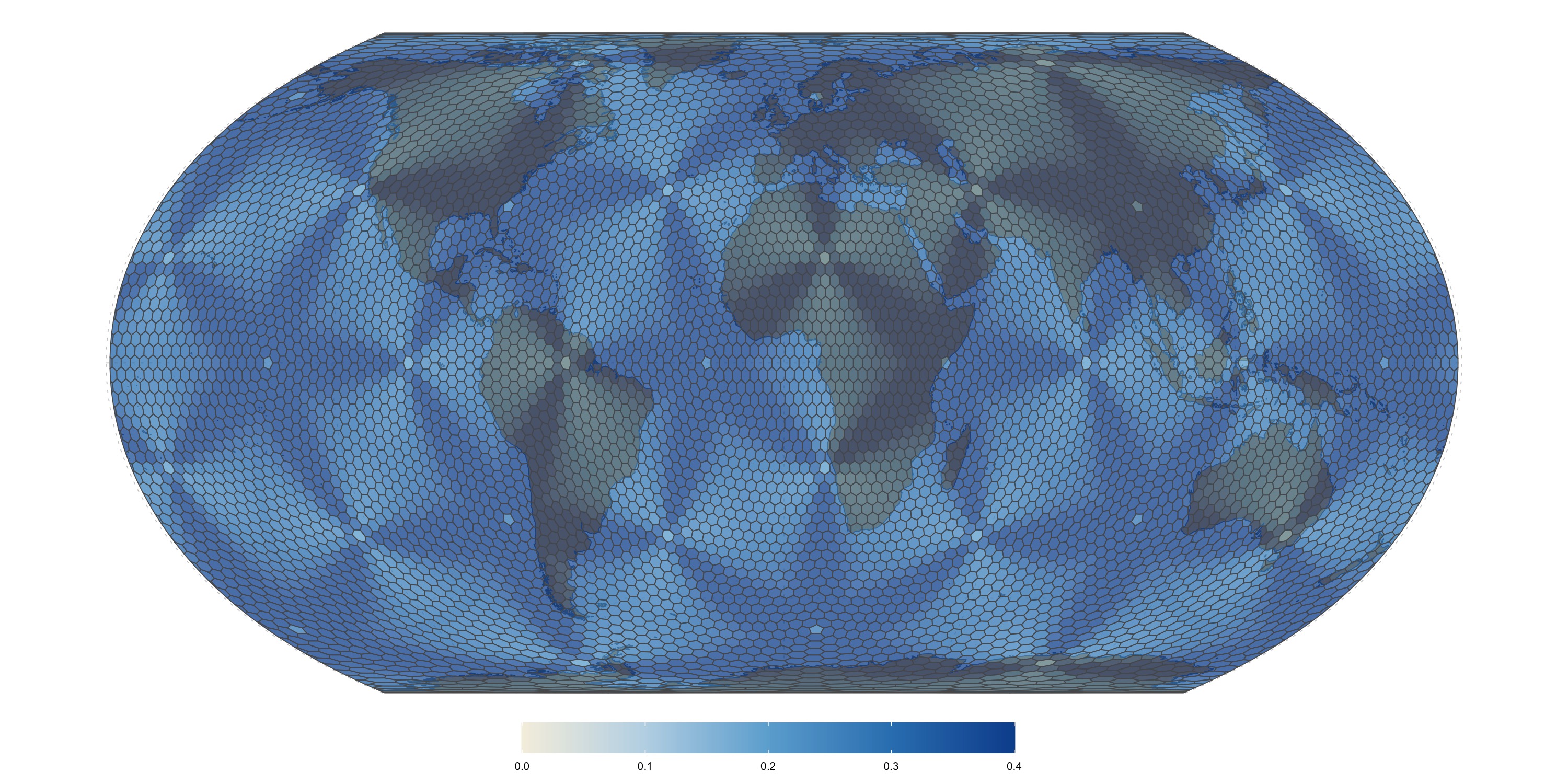
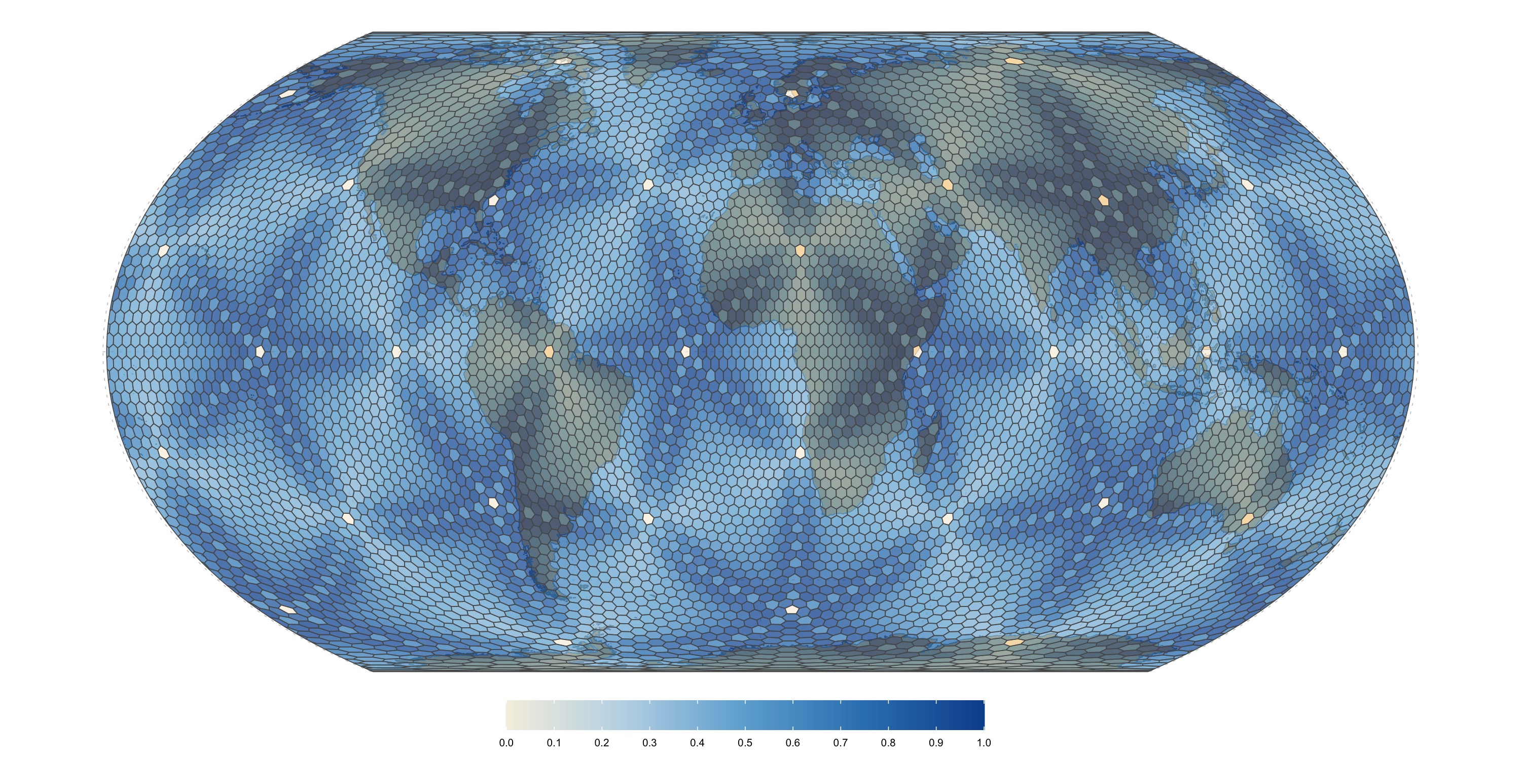
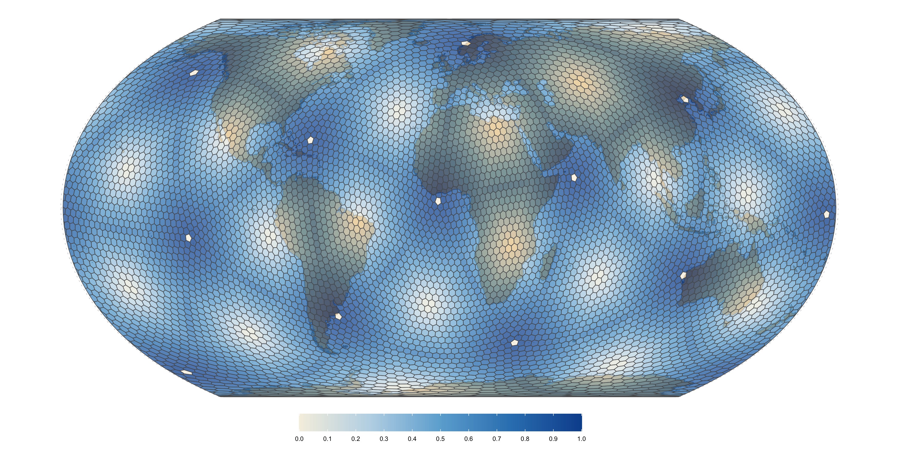
Variability in between-cell spacing (distance to adjacent cell centroids), calculated as the maximal deviation from the average neighbour spacing for each cell, and normalized by the maximal deviation across all cells. Values of zero mean no deviation, while values of 1 mean maximal deviation. Note that this is meant to visualize the areas with most distortion and high relative distortion does not mean high absolute distortion (in fact, for all surveyed grids the deviation in cell spacing is less than \(10%\))
ISEA (DGGAL) level 6 grid
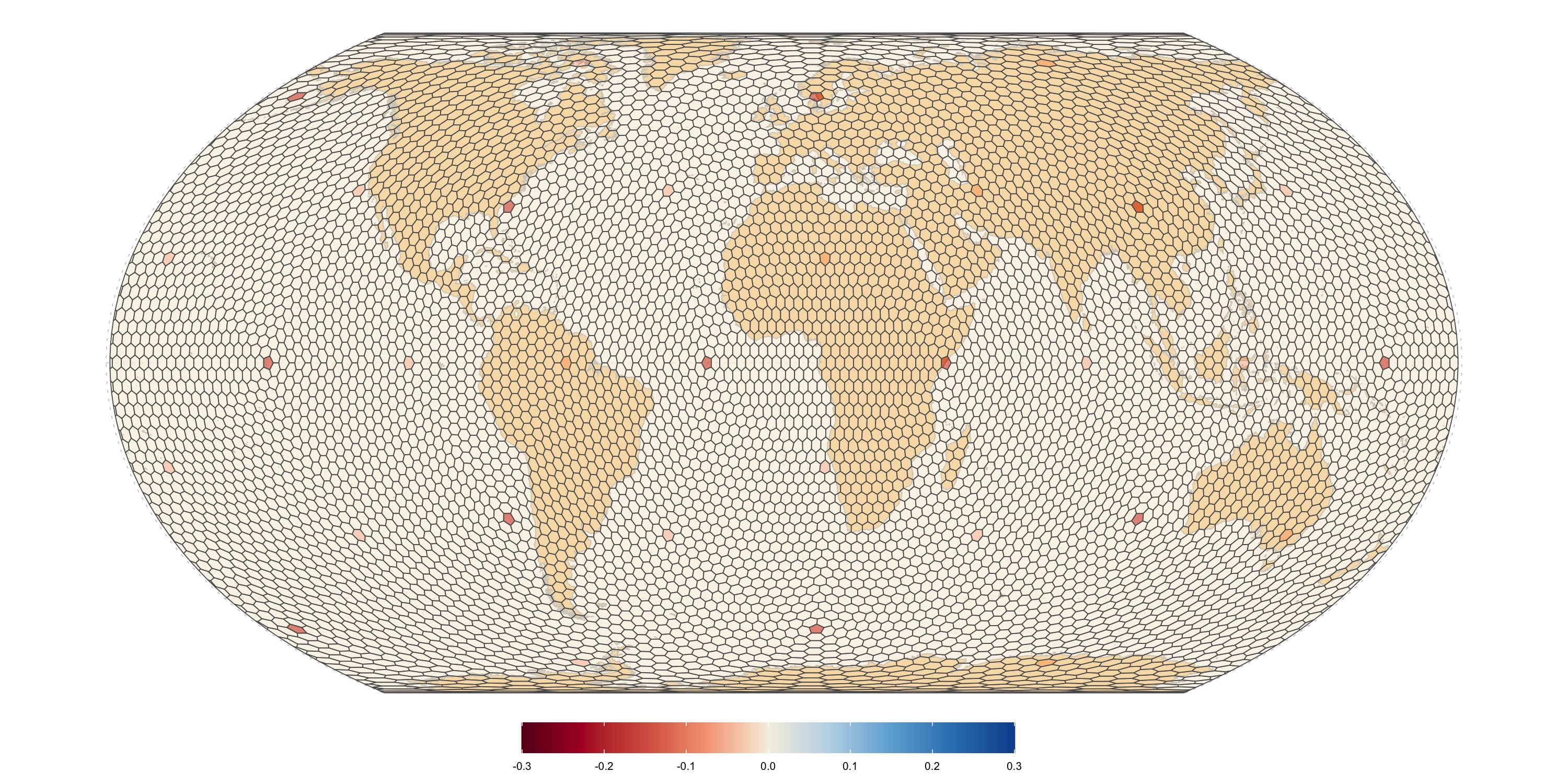
Area distortion relative to the mean. Values closer to zero mean less relative distortion.
Radial distortion calculated as ratio of largest to smallest distances between the centroid and the base cell boundary vertices, minus one. Zero means perfect radial symmetry.
Edge length distortion calculated as ratio of largest to smallest distances between adjacent base cell boundary vertices, minus one. Zero means that all edges have the same length.

Variability in between-cell spacing (distance to adjacent cell centroids), calculated as the maximal deviation from the average neighbour spacing for each cell, and normalized by the maximal deviation across all cells. Values of zero mean no deviation, while values of 1 mean maximal deviation. Note that this is meant to visualize the areas with most distortion and high relative distortion does not mean high absolute distortion (in fact, for all surveyed grids the deviation in cell spacing is less than \(10%\))
ISEA (dggridR) level 6 grid
Area distortion relative to the mean. Values closer to zero mean less relative distortion.
Radial distortion calculated as ratio of largest to smallest distances between the centroid and the base cell boundary vertices, minus one. Zero means perfect radial symmetry.
Edge length distortion calculated as ratio of largest to smallest distances between adjacent base cell boundary vertices, minus one. Zero means that all edges have the same length.
Variability in between-cell spacing (distance to adjacent cell centroids), calculated as the maximal deviation from the average neighbour spacing for each cell, and normalized by the maximal deviation across all cells. Values of zero mean no deviation, while values of 1 mean maximal deviation. Note that this is meant to visualize the areas with most distortion and high relative distortion does not mean high absolute distortion (in fact, for all surveyed grids the deviation in cell spacing is less than \(10%\))
Fuller uniform grid (300km)
Area distortion relative to the mean. Values closer to zero mean less relative distortion.
Radial distortion calculated as ratio of largest to smallest distances between the centroid and the base cell boundary vertices, minus one. Zero means perfect radial symmetry.
Edge length distortion calculated as ratio of largest to smallest distances between adjacent base cell boundary vertices, minus one. Zero means that all edges have the same length.
Variability in between-cell spacing (distance to adjacent cell centroids), calculated as the maximal deviation from the average neighbour spacing for each cell, and normalized by the maximal deviation across all cells. Values of zero mean no deviation, while values of 1 mean maximal deviation. Note that this is meant to visualize the areas with most distortion and high relative distortion does not mean high absolute distortion (in fact, for all surveyed grids the deviation in cell spacing is less than \(10%\))
Discussion and Conclusions
The results suggest that IVEA grids are a direct upgrade to the Snyder Equal-Area grids. IVEA features better worst-case area uniformity and more consistent spacing while retaining excellent edge length symmetry. In addition, irregularities are more smoothly distributed across the IVEA grid, rather than presenting as regions of high discontinuity, as in other methods. The tradeoff is slightly fewer regular cells (as indicated by higher radial asymmetry) — which appears to be a feature of the DGGAL implementation (as their ISEA grid is also slightly more uniform but has worse radial symmetry compared to the grid grids using the same projection). The uniform Fuller grid offers very high radial symmetry and excellent spacing uniformity but suffers from considerably higher area and edge length variability.
Additional advantages of IVEA and ISEA grids as implemented by DGGAL are that they are based on open standards and a shared global reference system. The position and properties of each cell are encoded in its unique identifier. This presents a strong argument for data reuse and compatibility between databases using the same grid system. Additionally, these grids enable cells at different levels to be related to one another. This enables adaptive approaches (varying grid resolution to provide more fidelity to areas of interest) and subsampling applications. In particular, in our work, we rely on subgrids to evaluate the dispersion of features across a cell (e.g., whether the feature is equally distributed across the entire cell or concentrated in a few locations).
Out of the 12 pentagon defects in the standard IVEA grid with a resolution of ~300km (level 6 grid), nine are located in the ocean. One defect is located off the coast of rural Sweden (approximately 150 km northwest of Gothenburg), one is off the coast of Somalia (approximately 100 km from Jilib), and one is in the mountains of Sichuan, China. Due to their remote location and (in most cases) position at the coast, none of these defects should pose any problems for practical applications.
References
1.
Goodchild, M. F. Geographical grid models for environmental monitoring and analysis across the globe (panel session). (1994).
2.
Kimerling, A. J., Sahr, K., White, D. & Song, L. Comparing geometrical properties of global grids. Cartography and Geographic Information Science 26, 271–288 (1999).
3.
St-Louis, J. & Corporation, E. DGGAL: Discrete global grid abstraction library. (2025).
4.
SNYDER, J. An equal-area map projection for polyhedral globes. Cartographica: The International Journal for Geographic Information and Geovisualization 29, 10–21 (1992).
5.
Leeuwen, D. van & Strebe, D. A" slice-and-dice" approach to area equivalence in polyhedral map projections. Cartography and Geographic Information Science 33, 269–286 (2006).
6.
Sahr, K. DGGRID: A command‐line application for generating and manipulating icosahedral discrete global grids. https://github.com/sahrk/DGGRID (2024).
7.
Barnes, R. & Sahr, K. dggridR: Discrete global grids for r. (2017).
8.
GRAY, R. Exact transformation equations for fuller’s world map. Cartographica: The International Journal for Geographic Information and Geovisualization 32, 17–25 (1995).
9.
Zakharko, T. Generating uniform geodesic grids for geospatial analyses. (2023).
10.
Rivière, P. The gray-fuller spatial grid.